Pattern Recognition and Machine Learning - Visualisations
Visualisations of different parts of the PRML book Pattern Recognition and Machine Learning by Christopher M. Bishop (2006).
The code can be found at https://github.com/Daniel-Sinkin/Deeplearning/
Table of Contents
- EM Algo
- Markov Chain Monte Carlo
- Rejection Sampling
- Ridge Regression
- Curve Fitting
- PCA
- Effect of Regularisation
- Box Muller
- Integral Density
- Gaussian Process
- References
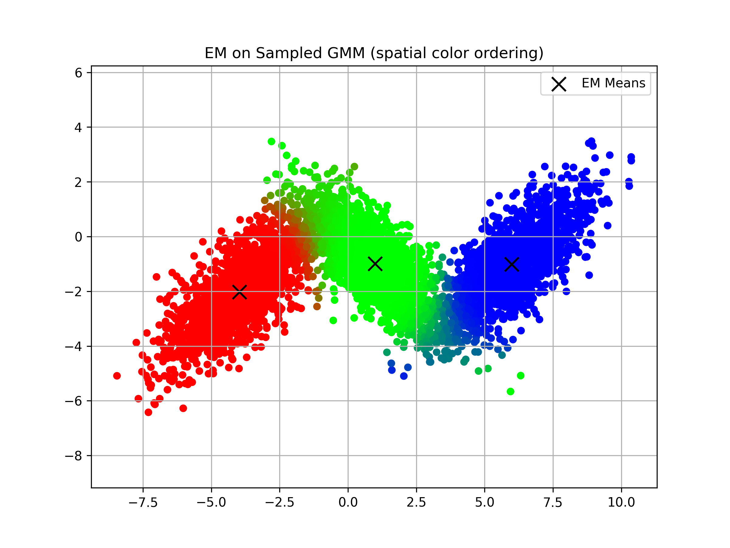
EM Algo
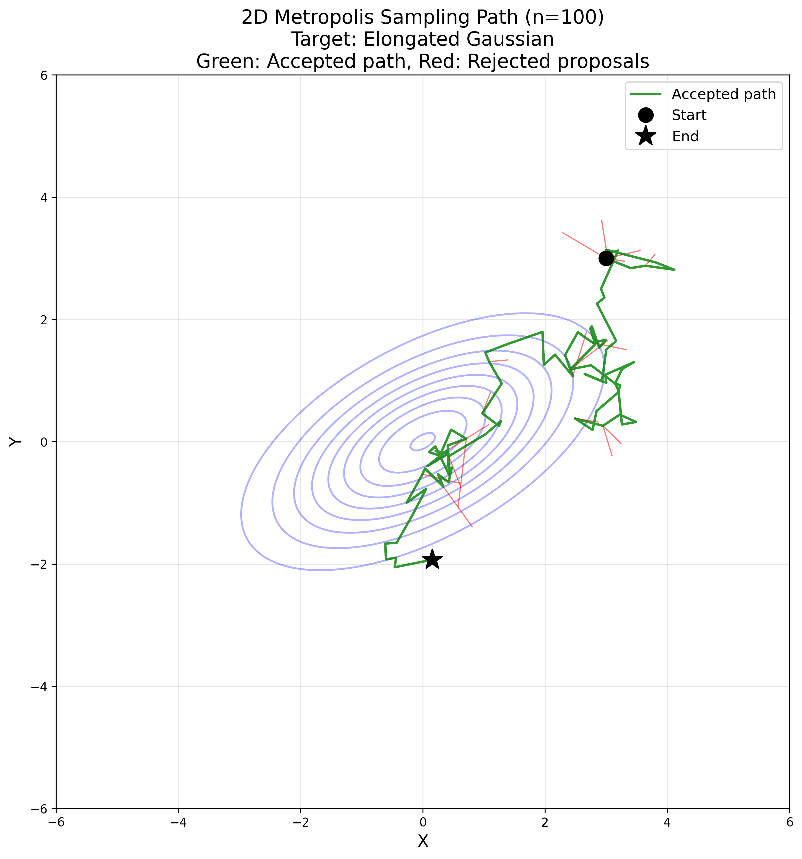
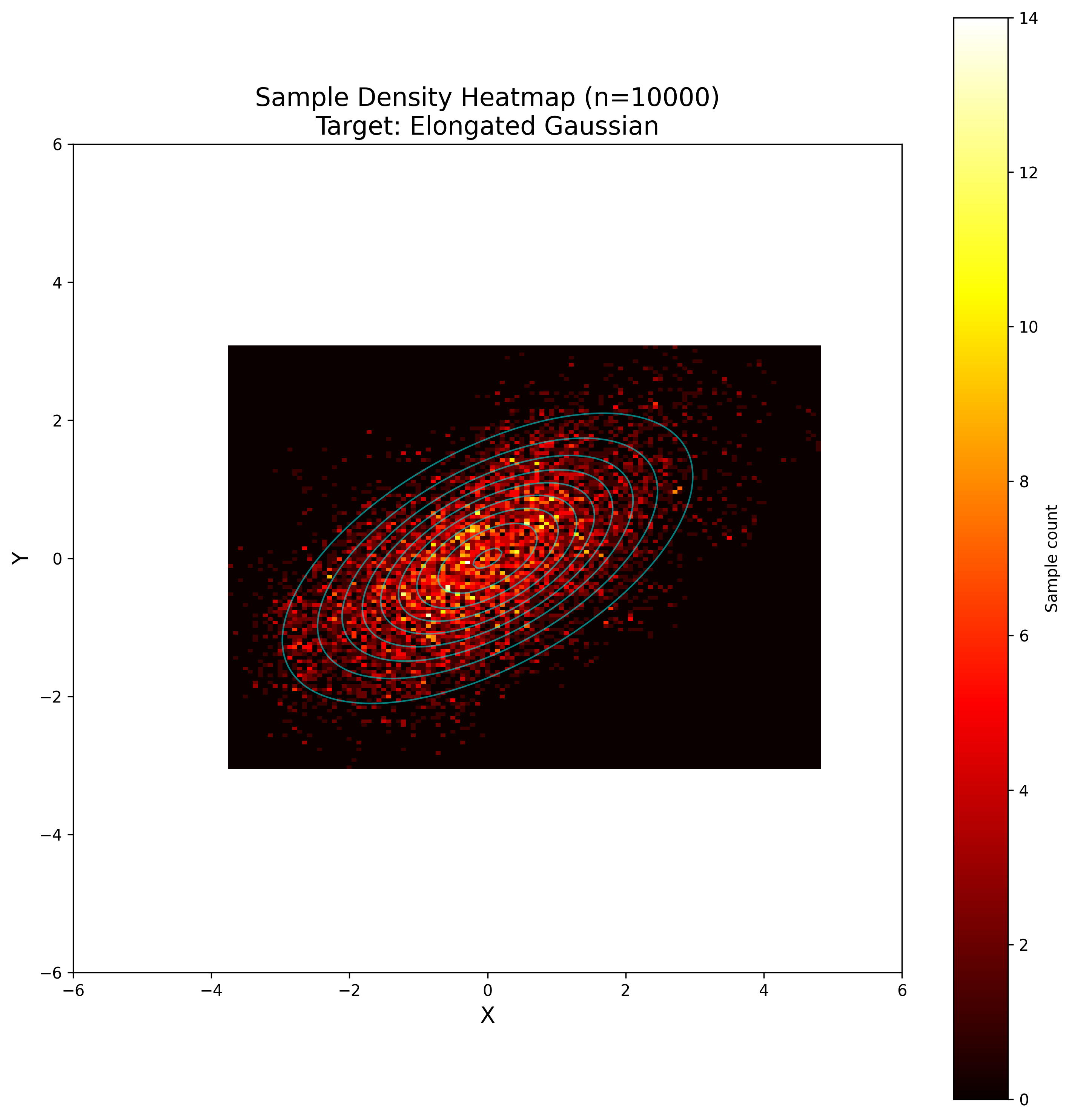
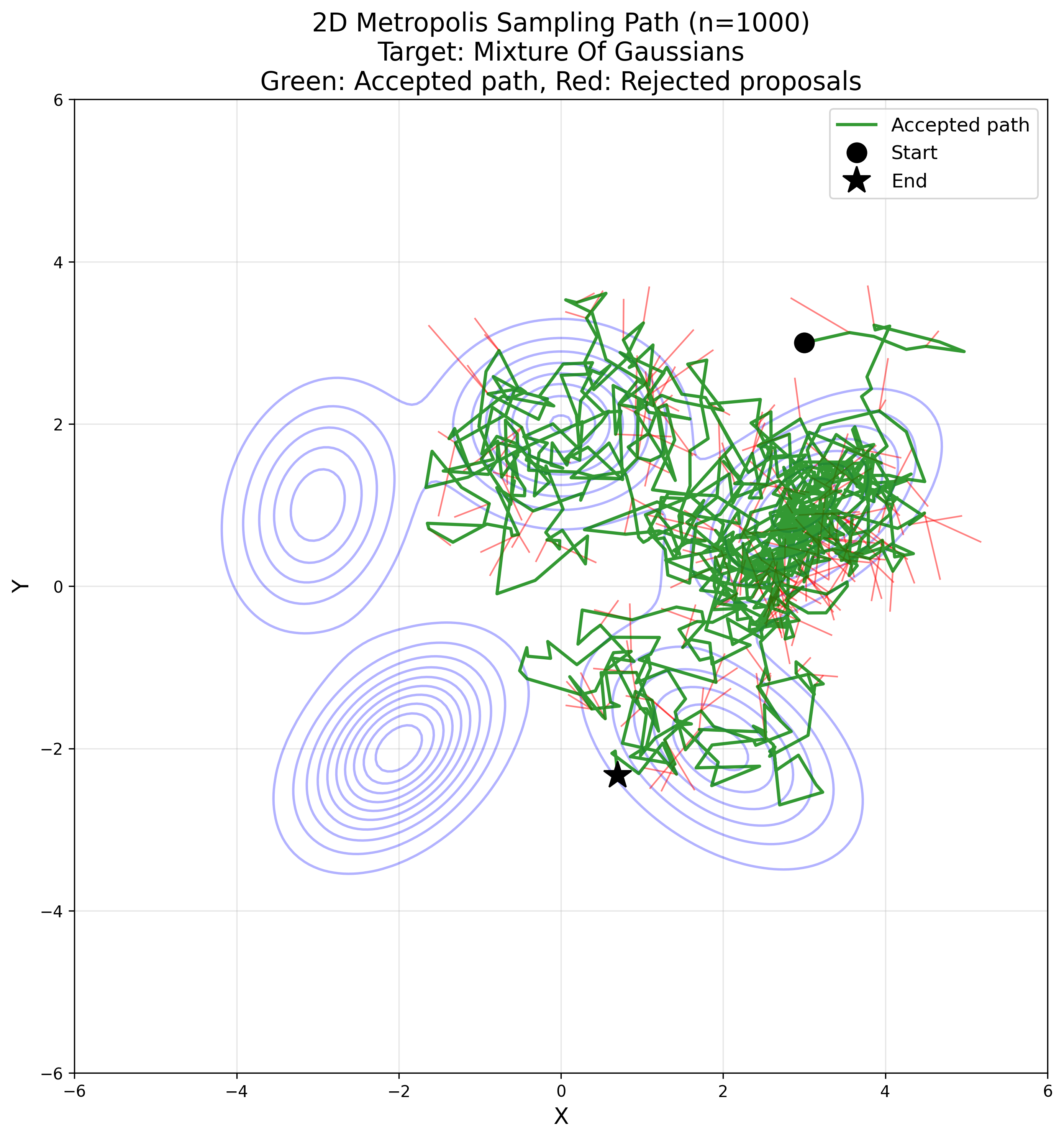
Markov Chain Monte Carlo
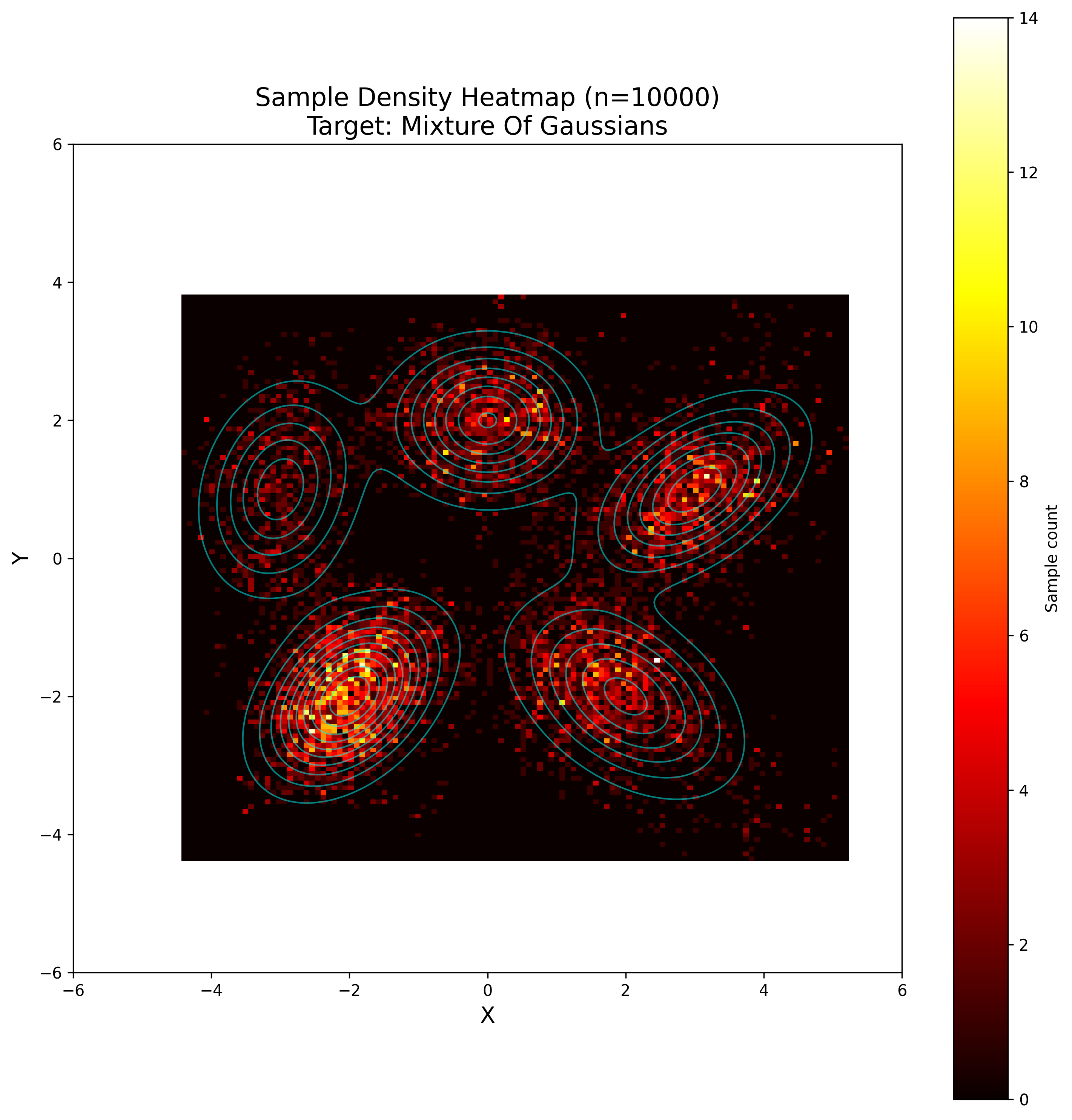
Suppose we have a sample point (in this example $z_t = (x_t, y_t) \in \mathbb{R}^2$), then we sample a pre-defined proposal distribution. For the basic Metropolis algorithm it needs to be symmetric, in the sense that
\[p(x|y) = p(y|x)\]holds. Isotropic multivariate Gaussian $\mathcal{N}(0, \sigma^2 I)$ and uniform distribution $U((-a, a) \times (-a, a))$ both satisfy this condition. For this example we are taking the Gaussian distribution as the proposal function.
We sample a direction $\delta \sim \mathcal{N}(0, \sigma^2 I)$ and for our target function (an unnormalised distribution) $\tilde{p}$ we compute the (possibly overflowing) acceptance value of this step as follows:
\[\tilde{A}(z_t, z_t + \delta) := \frac{p(z_t + \delta)}{p(z_t)},\]As we want an acceptance probability, we need to clip it to be at most 1:
\[A(z_t, z_t + \delta) = \min(1, \tilde{A}(z_t, z_t + \delta)) = \min\left(1, \frac{p(z_t + \delta)}{p(z_t)}\right)\]We then accept this step with probability $A(z_t, z_t + \delta)$, by sampling
\[u \sim U(0, 1)\]and checking if $u \leq A(z_t, z_t + \delta)$ (which of course is always the case if $\tilde{A}(z_t, z_t + \delta) \geq 1.0$).
If we accept, we define $z_{t + 1} = z_t + \delta$; otherwise, we simply remain at the same position, i.e., $z_{t + 1} = z_t$.
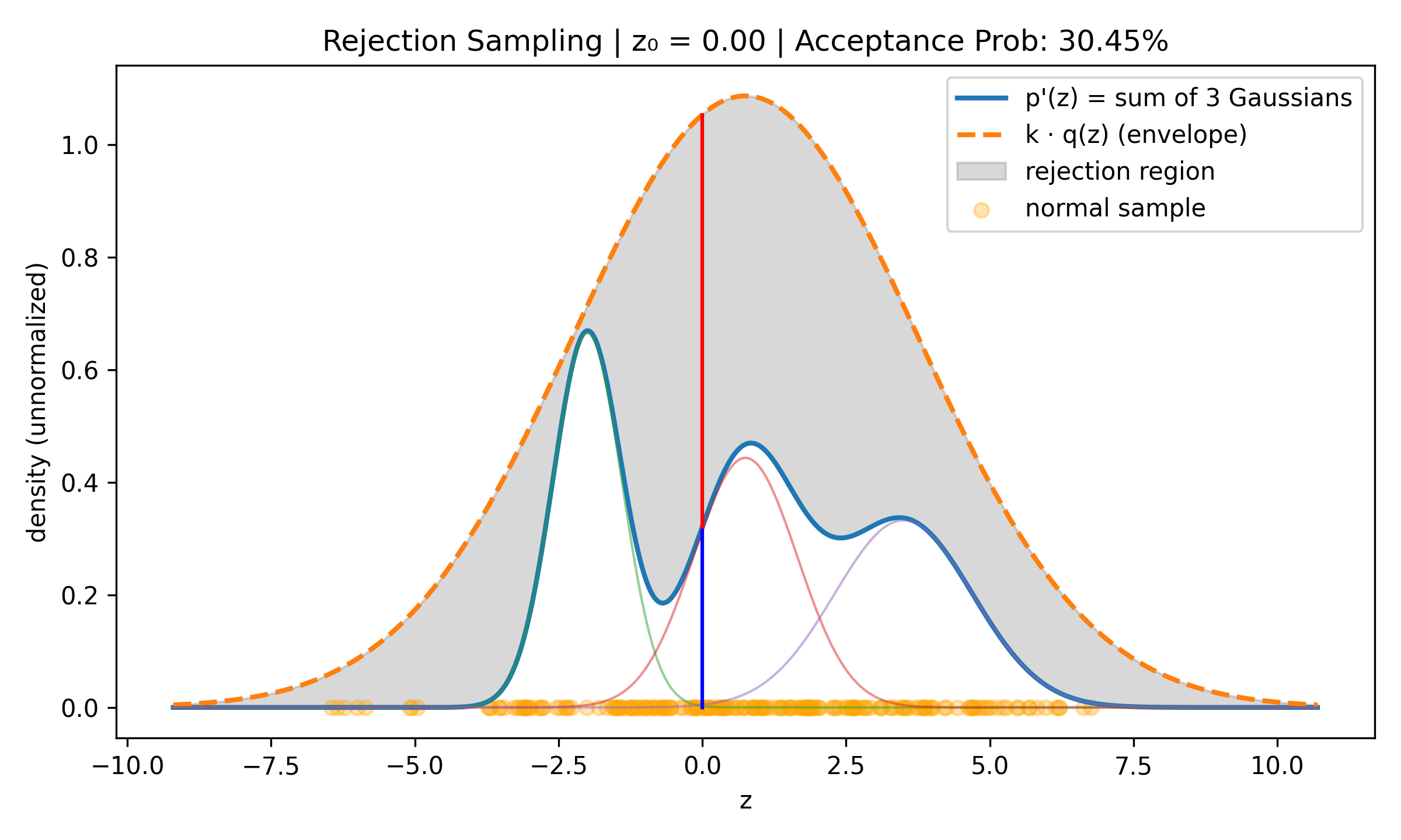
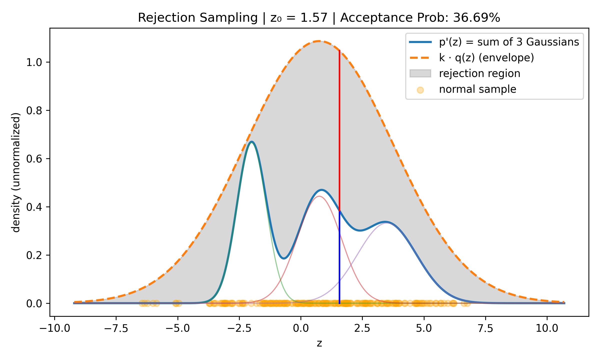
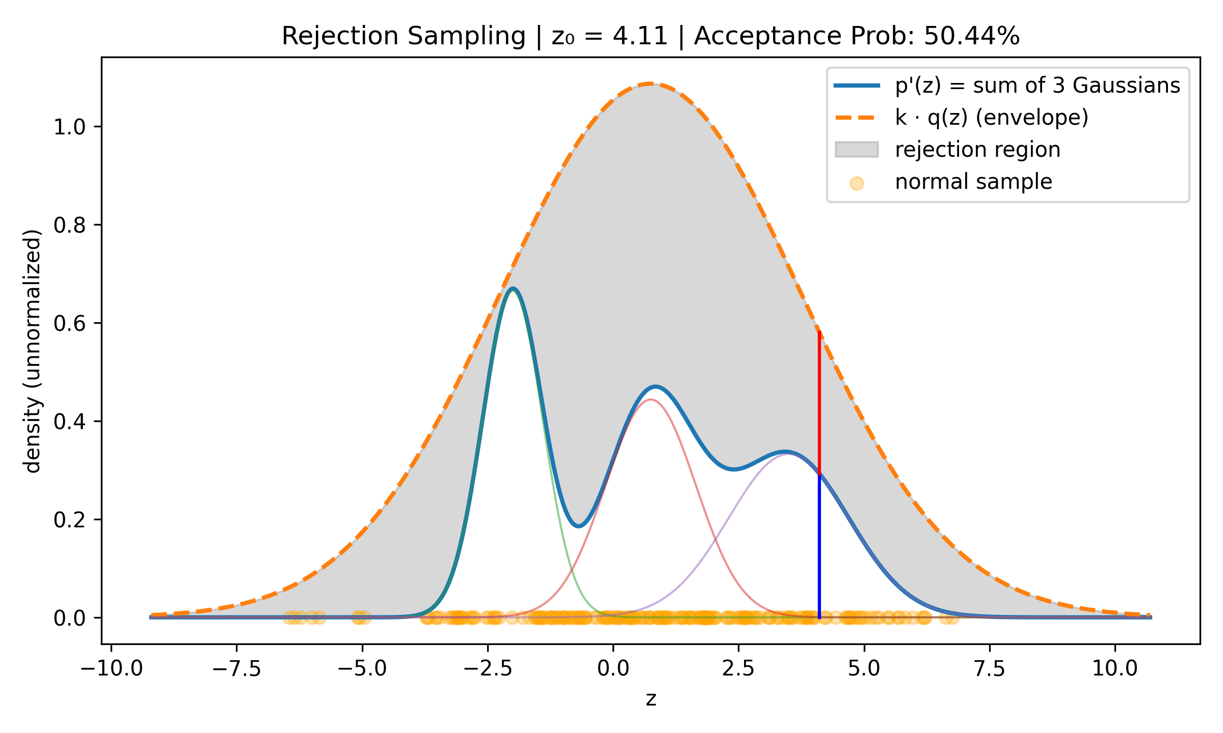
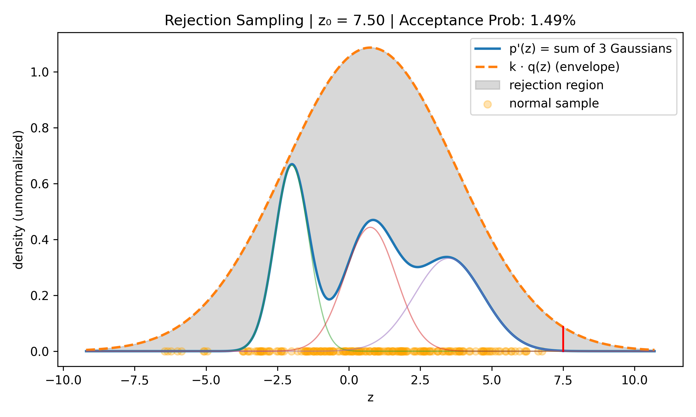
Rejection Sampling
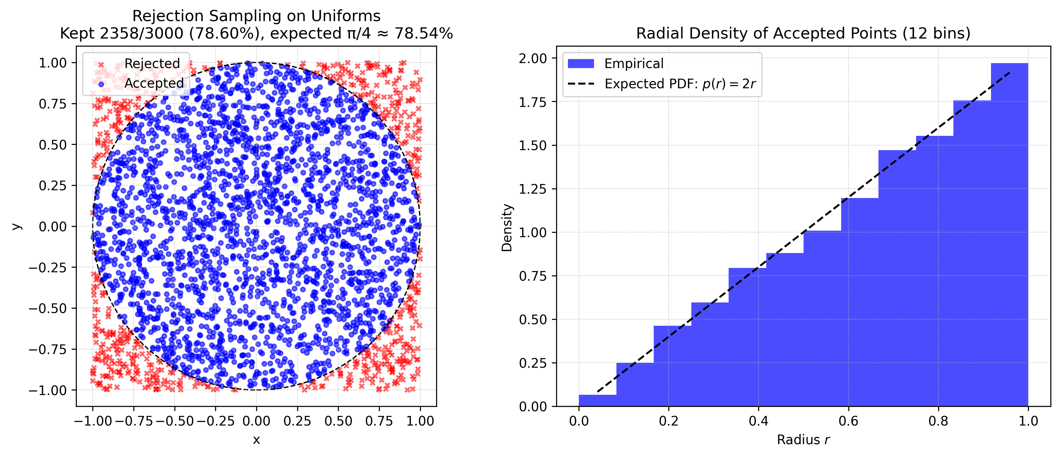
Suppose we want to sample a complex distribution \(p(z)\) what is easy to evaluate if we ignore normalisation, i.e., such that \(\tilde{p}(z) = C p(z)\) C > 0 is easy to evaluate. Take some simple to evaluate distribution \(q(z)\) (for example normal) and find \(k > 0\) such that \(kq(z) > \tilde{p}(z)\) for all \(z\). Then do uniform sampling on \(\xi \sim U(0, kq(z_0))\) and accept if \(\xi \leq \tilde{p}(z)\), reject otherwise. The acceptance rate is proportional to \(\frac{1}{k}\) so we want to have k as small as possible.
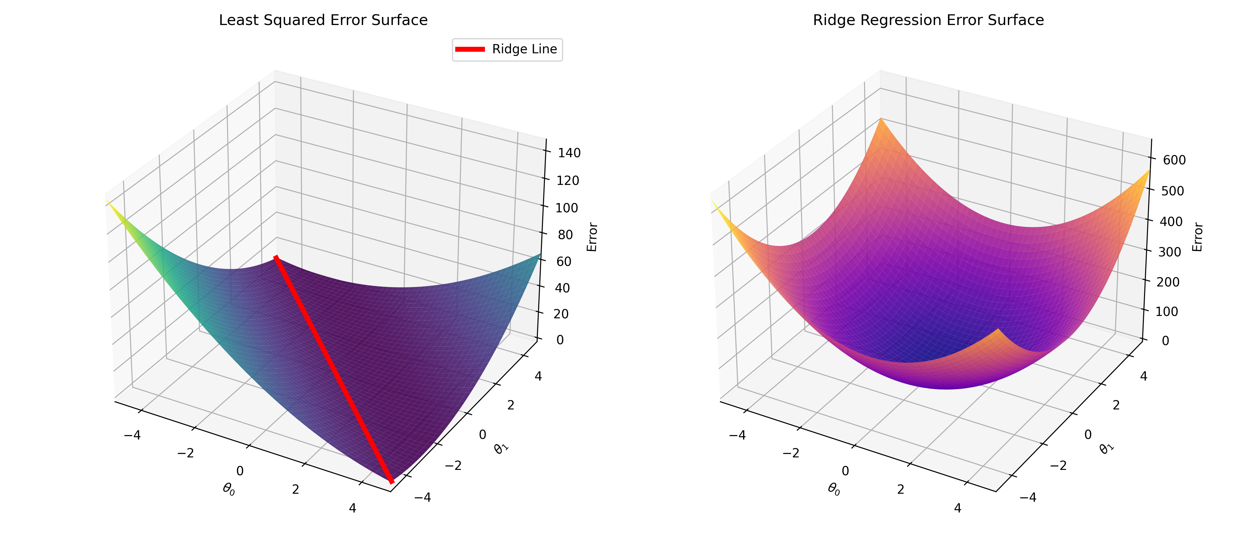
Ridge Regression
Here I implemented the discussion in this stackexchange answer https://stats.stackexchange.com/a/151351
which shows the “Ridge” that we get with overfitting explicitly
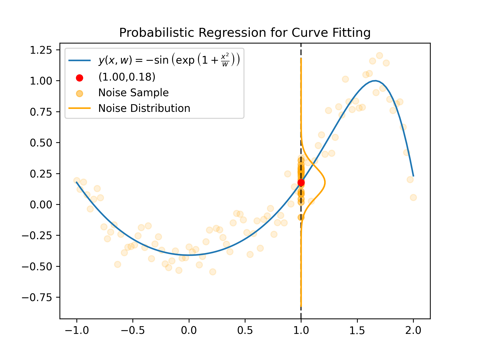
Curve Fitting
Assuming we are fitting a curve with Gaussian Noise, then for any fixed x value the distribution
of the target value is given as follows (based on Figure 1.28 in Bishop, Pattern Recognition and Machine Learning, 2006)
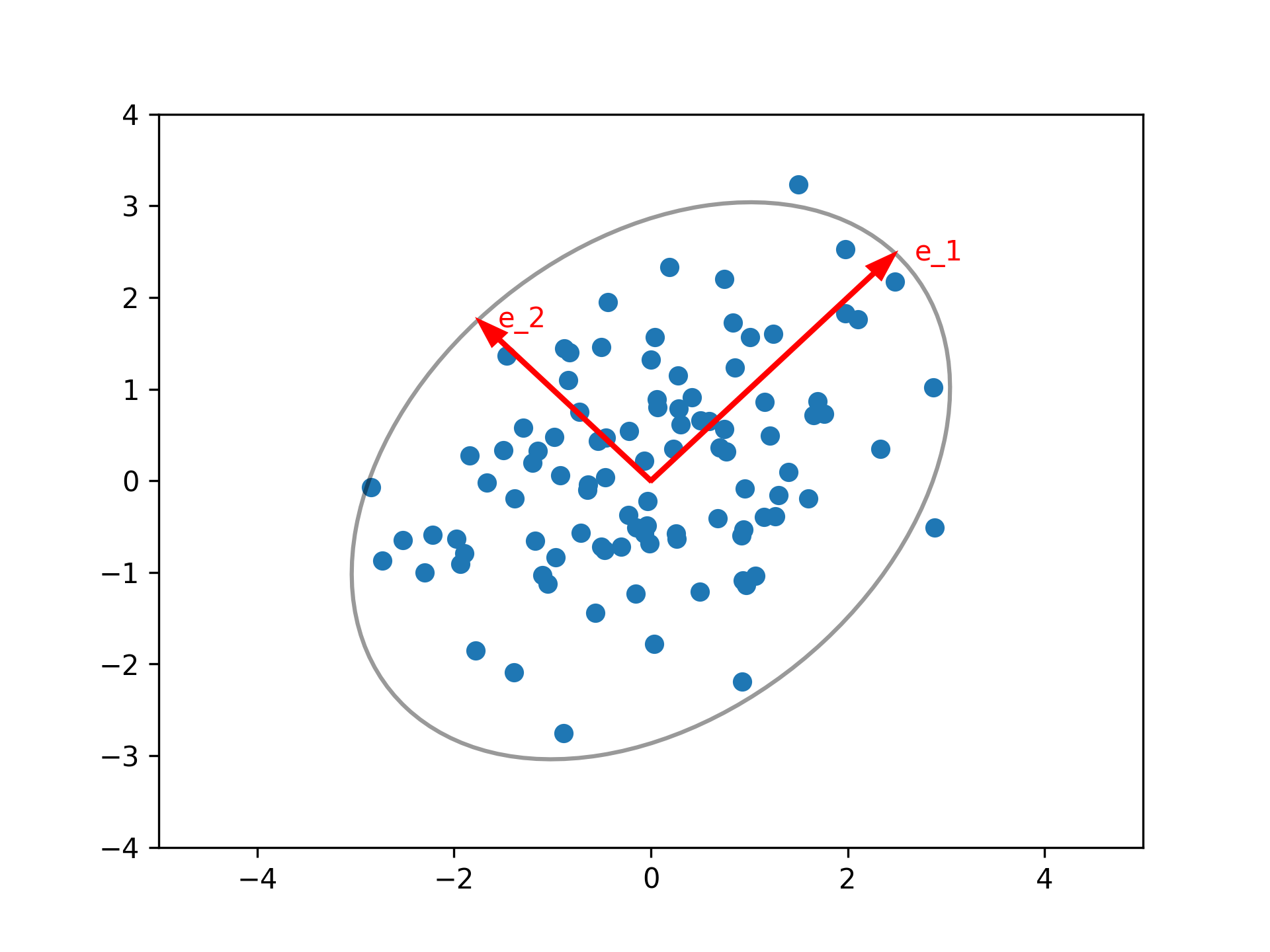
PCA
We take our samples \(X = \{x_1, \dots, x_N\} \subseteq \mathbb{R}^D\) and construct the covariance matrix \(\Sigma_X = \sum_{i = 1}^N x_i^\top x_i\). This is a symmetric positive definite matrix (assuming all samples are linearly independent) as such it has \(N\) eigenvectors \(v_1, \dots, v_N\) and \(n\) positive (!) eigenvalues \(\lambda_1, \dots, \lambda_N\), without loss of generality we can assume that \(\lambda_1 \geq \lambda_2 \geq \dots \lambda_N\).
The first \(k\) eigenvectors then give us the most important to extract the most important components
Effect of regularisation
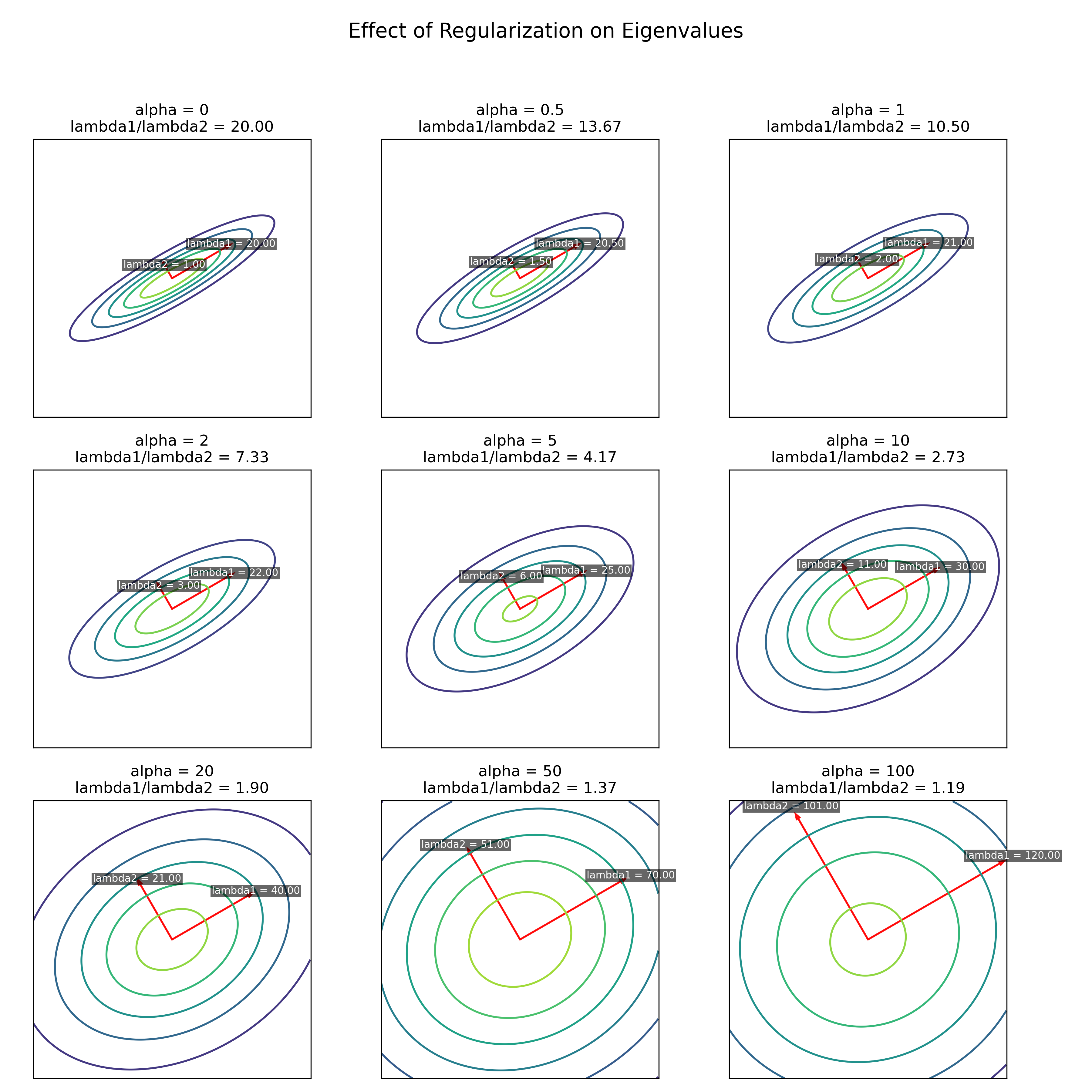
Suppose we have a covariance matrix \(\Sigma \in \mathbb{R}^{N \times N}\), we can regularise by
making the diagonal more dominant, applying so-called Tychonoff (or Tikhonov) Regularisation: \(\Sigma_\alpha = \alpha I_{N \times N} + \Sigma\)
The effect of this is it makes the underlying equicontours more spherical, in the sense that
the eigenvalues are closer together (\(\lambda_i / \lambda_{i + 1}\) goes closer to 1)
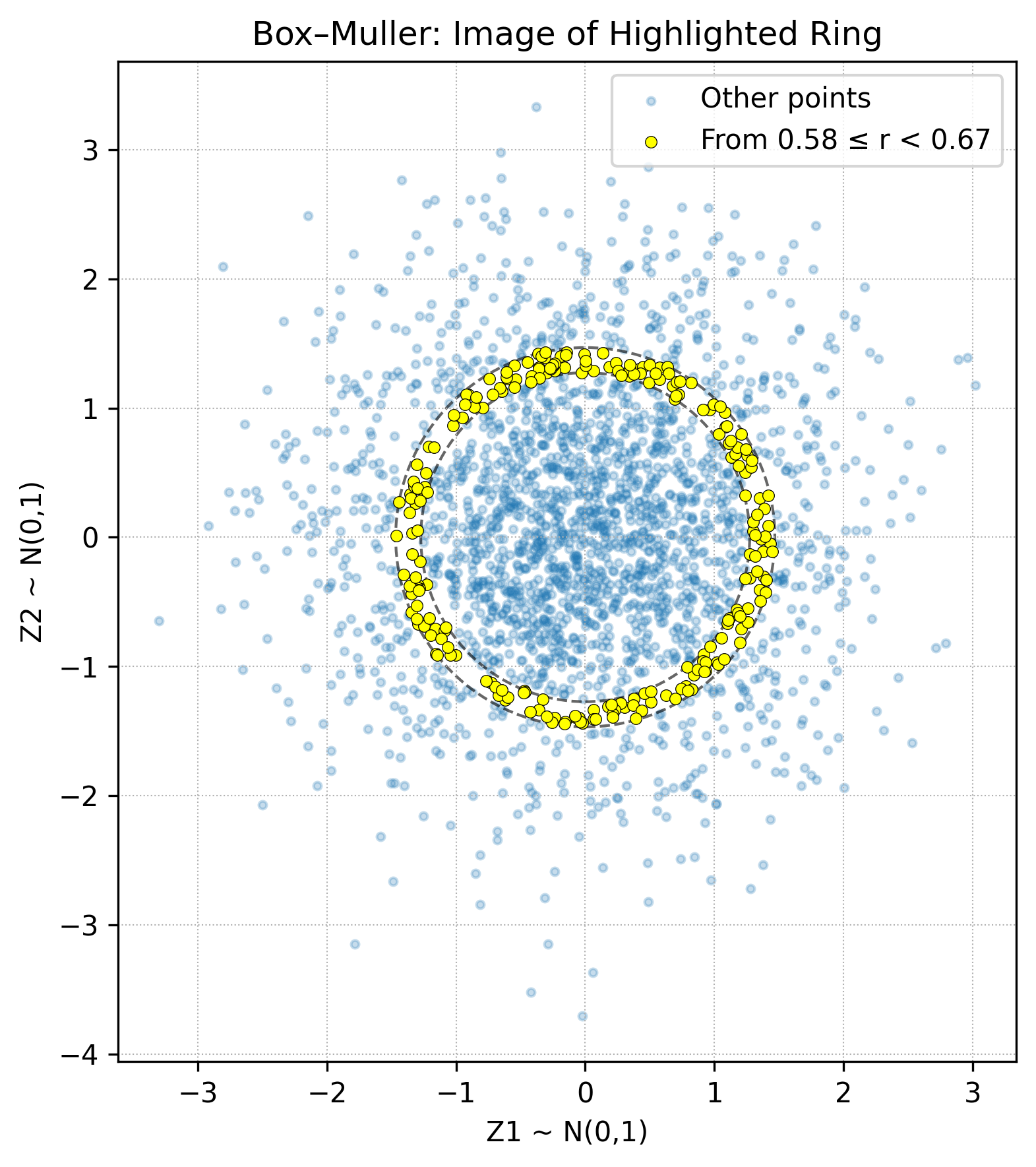
Box Muller
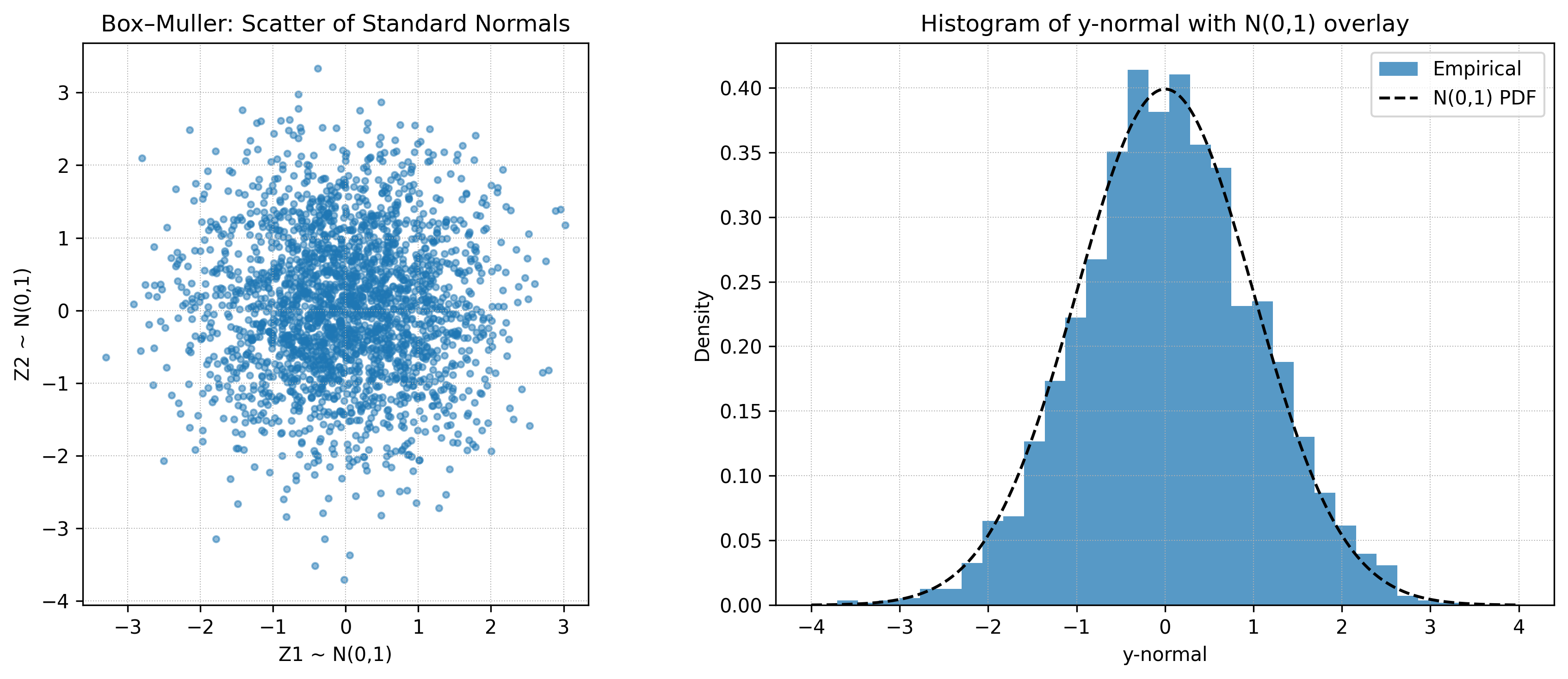
A somewhat efficient algorithm for sample standard normal random variable using a transform on uniforms distributed variables. Suppose we want to sample \(2N\) standard normal variables.
First start with \(X^{(0)} := \{(x_i, y_i) : 1 \leq i \leq N\}\) random variables such that \(x_i, y_i \sim U(0, 1)\)
and reject all samples where \(r_i^2 := x_i^2 + y_i^2 > 1.0,\)
giving us \(X^{(1)} = \{(x_i, y_i) \in X : r_i^2 \leq 1.0\}.\)
 We then apply the transform \(s_i^{(1)} = x_i \sqrt{\frac{-2\log(r_i^2)}{r_i^2}}\) and \(s_i^{(2)} = y_i \sqrt{\frac{-2\log(r_i^2)}{r_i^2}}\) it can be shown that \(s_i^{(1)}\) and \(s_i^{(1)}\) are iid with \(s_i^{(j)} \sim \mathcal{N}(0, 1)\).
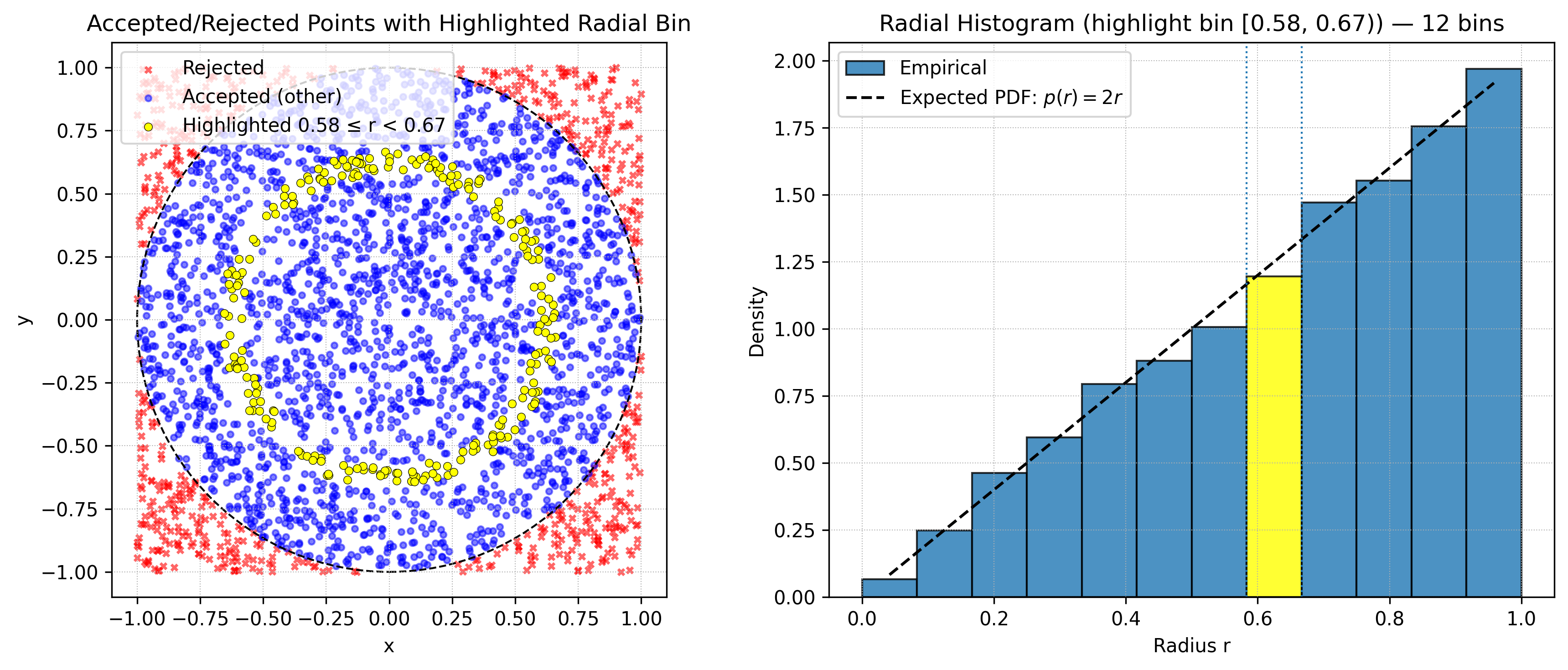
 This uses the rotational symmetry of the 2 dimensional normal distribution. We can see more accurately
what the transformation does by highlighting a particular slice
This uses the rotational symmetry of the 2 dimensional normal distribution. We can see more accurately
what the transformation does by highlighting a particular slice
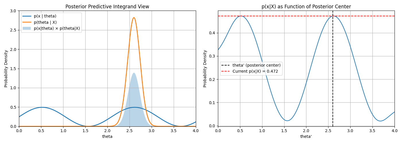
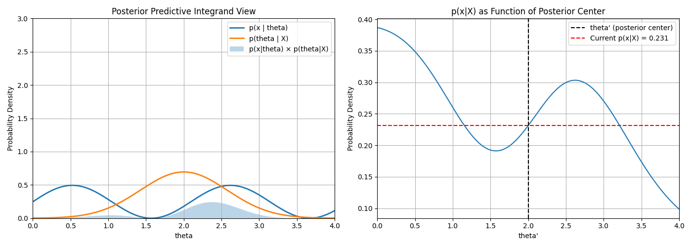
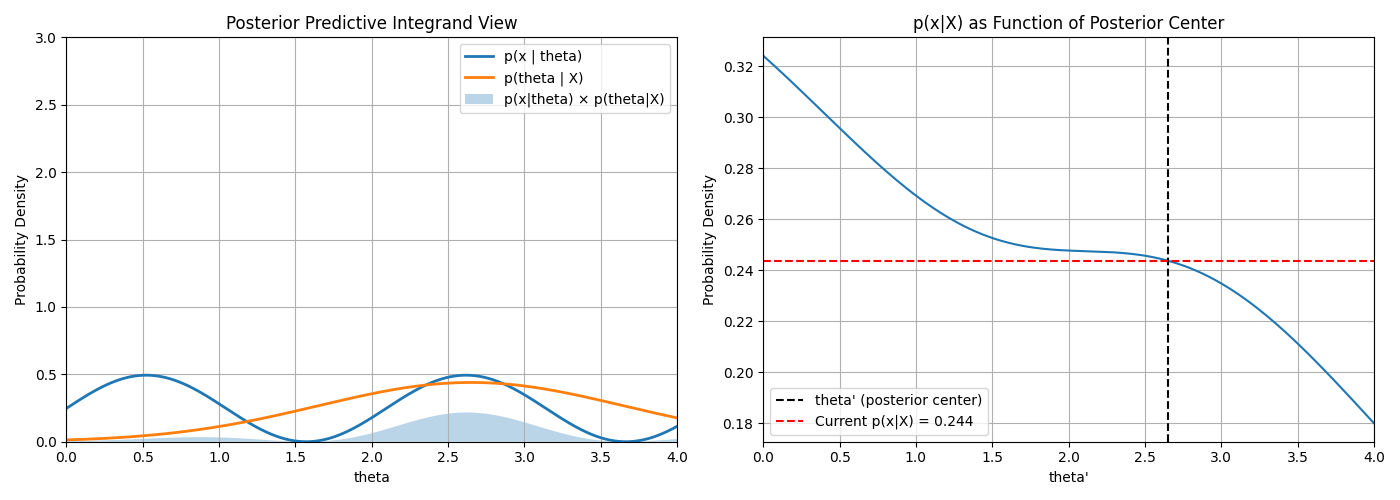
Integral Density
When doing Bayesian inference, if \(p(\hat{\theta}|x)\) is very close to 1 for a particular \(\hat{\theta}\)
and close to \(0\) for all others then \(p(x|X) \approx p(X|\hat{\theta})\)
This visualises this phenomonon
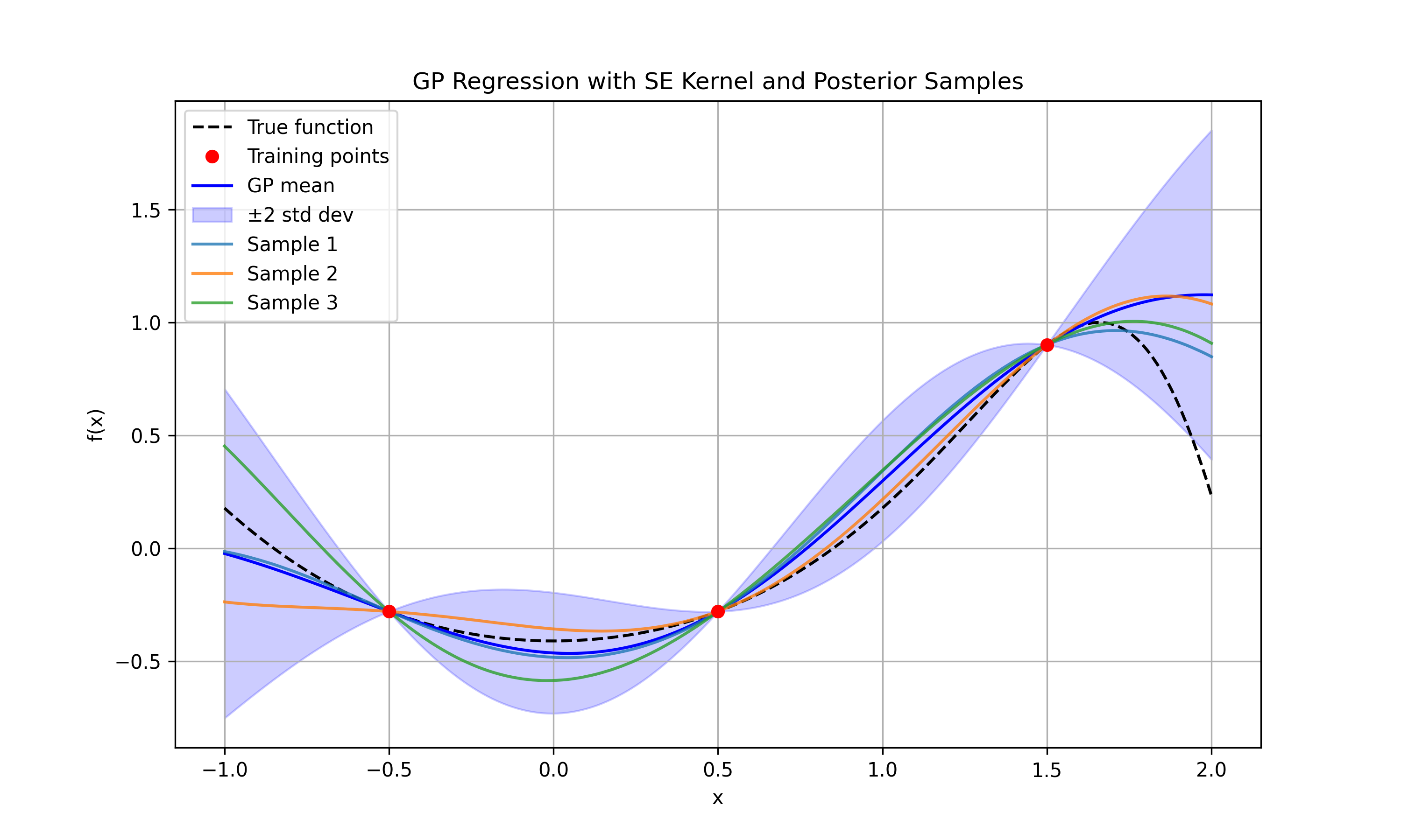
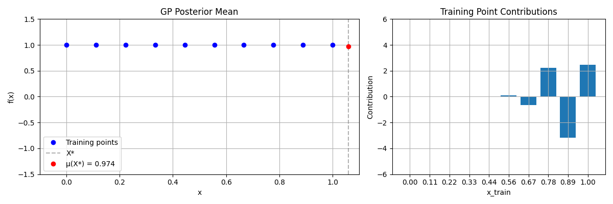
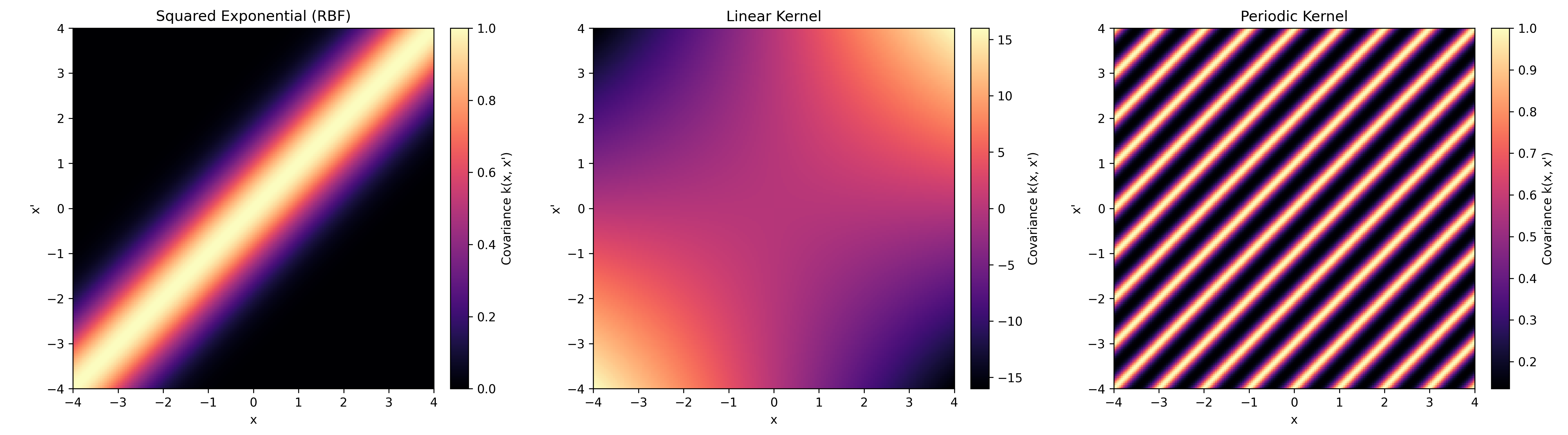
Gaussian Process
Normal
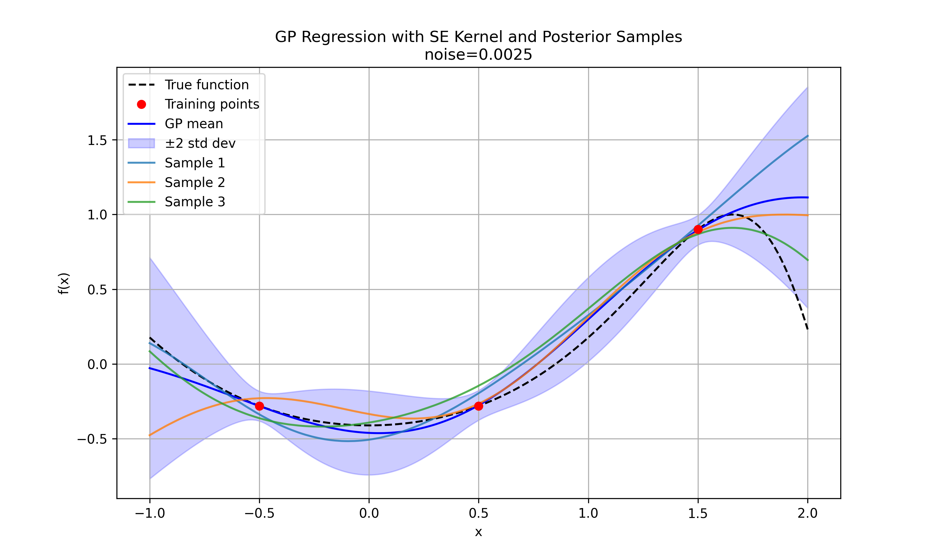
 With added noise
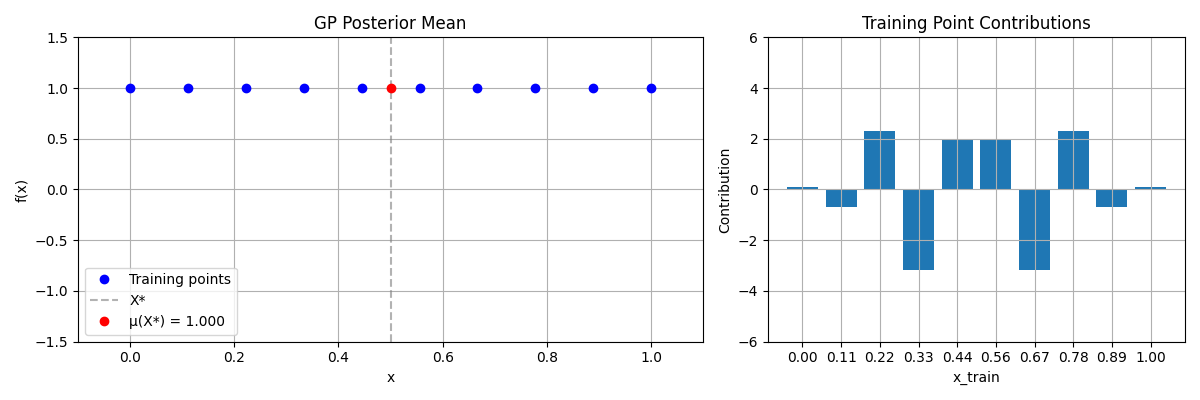
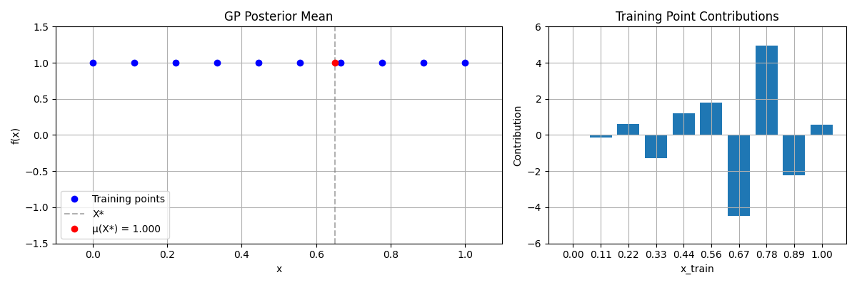
Contribution Histograms
Heatmap of different Kernels
References
- Bishop, C. M. (2006). Pattern Recognition and Machine Learning. Springer.