Geometry of Linear Regression
Let
\[\phi : S \rightarrow T\]be a transformation (for example $S = \mathbb{R}^m, T = \mathbb{R}^D$) and suppose we are given training samples \(\{(x_i, t_i) : 1 \leq i \leq N\}\), where $x_i \in S$. We define a generalized linear regression function by
\[y(x, w) = w^t\phi(x) \in \mathbb{R},\]where
\[w = \begin{pmatrix} w_1 \\ w_2 \\ \vdots \\ w_D \end{pmatrix} \in \mathbb{R}^D\]approximates the training data, in the sense that the $L^2$ distance between the \(y(x_i, w)\) and \(t_i\) is minmal, i.e., we want to find
\[w_\text{opt} = \arg \min_{w \in \mathbb{R}^D} \sum_{i = 1}^N ||y(x_i, w) - t_i||^2.\]We call
\[\sum_{i = 1}^N ||y(x_i, w) - t_i||^2\]the least squares loss. We write
\[\Phi(x) = (\phi(x_1), \phi(x_2), \dots \phi(x_K)) \in \mathbb{R}^{D \times K}\]Example
Let \(T = \mathbb{R}^2\) and suppose we have samples $x_1, x_2, x_3$ such that
\[\begin{aligned} \phi(x_1) = \begin{pmatrix} 1 \\ 0\end{pmatrix},&& \phi(x_2) = \begin{pmatrix} 0 \\ 1\end{pmatrix},&& \phi(x_3) = \begin{pmatrix} 1 \\ 1\end{pmatrix}. \end{aligned}\]and our corresponding targets are \(t_1 = 1, t_2 = 1, t_3 = 0\), then our least squares regression has the form
\[\begin{aligned} E(w) &= ||w^t\phi(x_1) - t_1||^2 + ||w^t\phi(x_2) - t_2||^2 + ||w^t\phi(x_3) - t_3||^2 \\ &= (w_1 - 1)^2 + (w_2 - 1)^2 + (w_1 + w_2)^2 \end{aligned}\]This gives us an explicit function to optimise:
\[f(x, y) = (x - 1)^2 + (y - 1)^2 + (x + y)^2\]note that it is strictly convex so all critical points will be minimizers:
\[\nabla f(x, y) = \begin{pmatrix} 2(x - 1) + 2(x + y) \\ 2(y - 1) + 2 (x + y) \end{pmatrix} \overset{!}{=} 0\]which is the case if and only if
\[\begin{aligned} 4x + 2y - 2 = 0,&&2x + 4y - 2 = 0 \end{aligned}\]which is a linear system with two unknowns and two equations, with full rank so we get a unique solution
\[x = 1/3, y = 1/3\]A more general approach to get to this solution is to set up the normal equation, to that end consider
\[\Phi(x) = (\phi_1(x), \phi_2(x), \phi_3(x)) = \begin{pmatrix} 1 && 0 && 1 \\ 0 && 1 && 1 \end{pmatrix} \in \mathbb{R}^{2 \times 3}\]and compute
\[\Phi(x) \Phi(x)^\top = \begin{pmatrix} 1 & 0 & 1 \\ 0 & 1 & 1 \end{pmatrix} \begin{pmatrix} 1 & 0 \\ 0 & 1 \\ 1 & 1 \end{pmatrix} = \begin{pmatrix} 2 & 1 \\ 1 & 2 \end{pmatrix}\]We compute
\[(\Phi(x) \Phi(x)^\top)^{-1}\Phi(x) \begin{pmatrix} 1 \\ 1 \\ 0\end{pmatrix} = \begin{pmatrix} 2 & 1 \\ 1 & 2 \end{pmatrix}^{-1} \begin{pmatrix} 1 & 0 & 1 \\ 0 & 1 & 1 \end{pmatrix} \begin{pmatrix} 1 \\ 1 \\ 0\end{pmatrix} = \begin{pmatrix} 1/3 \\ 1/3 \end{pmatrix}\]Example 2
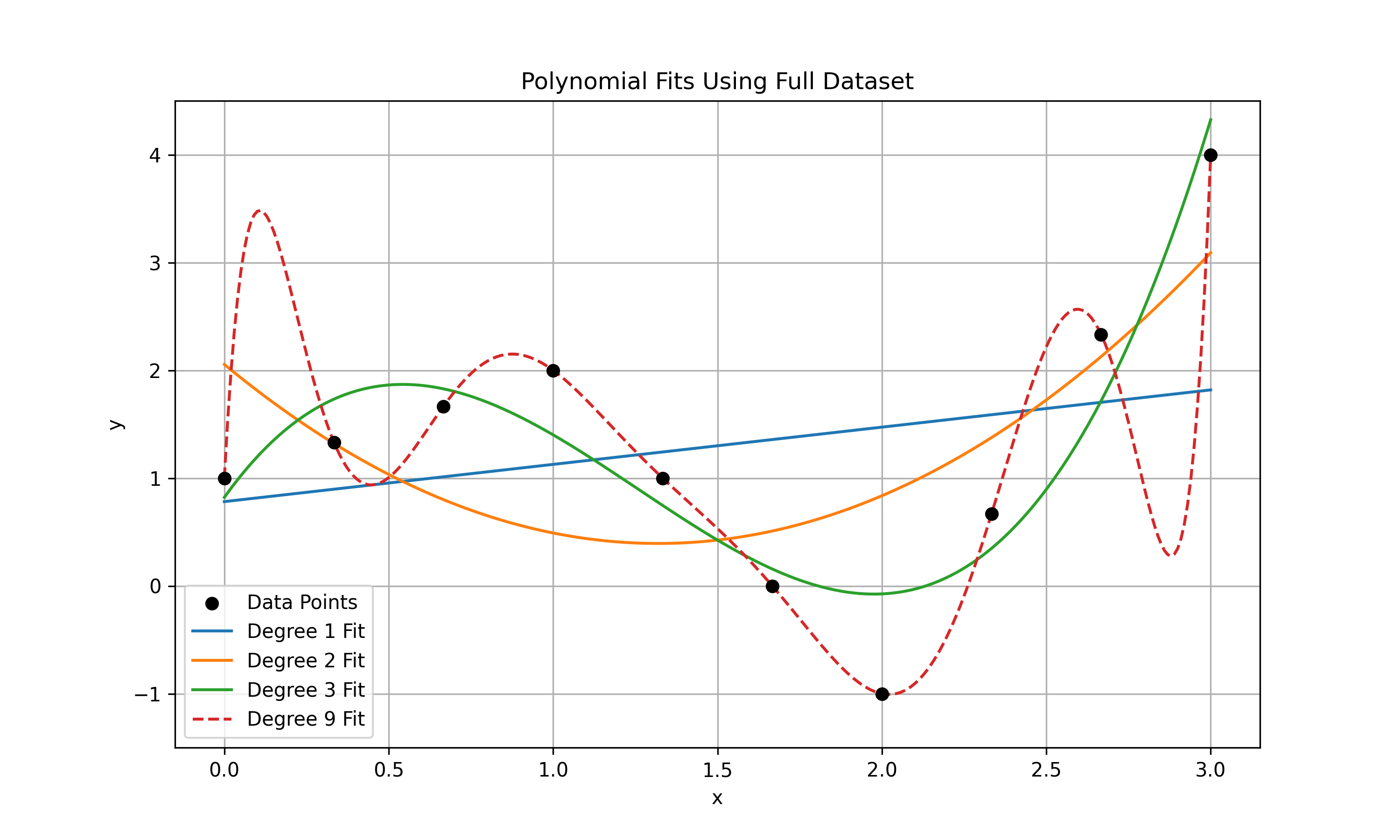
We want to polynomial fit the points $(x_i, y_i)$ given by
\[\left(0, 1\right),\ \left(\frac{1}{3}, \frac{4}{3}\right),\ \left(\frac{2}{3}, \frac{5}{3}\right),\ \left(1, 2\right),\ \left(\frac{4}{3}, 1\right),\ \left(\frac{5}{3}, 0\right),\ \left(2, -1\right),\ \left(\frac{7}{3}, \frac{2}{3}\right),\ \left(\frac{8}{3}, \frac{7}{3}\right),\ \left(3, 4\right)\]using polynomials, given that we have two changes in direction ($y_1 < y_2, y_2 > y_3, y_3 < y_4$) it makes sense to use a polynomial of degree 3, i.e., defined via the basis
\[\begin{aligned} \phi_0(x) = 1,&&\phi_1(x) = x,&&\phi_2(x) = x^2,&&\phi_3(x) = x^3 \end{aligned}\]defining the linear regression function
\[y(x, w) = w^t\Phi(x)\] \[\begin{aligned} y(x, w) &= w_0 \phi_0(x) + w_1 \phi_1(x) + w_2 \phi_2(x) + w_3 \phi_3(x) \\ &= w_0 + w_1 x + w_2 x^2 + w_3 x^3 \end{aligned}\]