This blog post goes through the details of how to sample a function using Gaussian Process, mostly based on Rasmussen & Williams (2006) Chapter 2 and on Bishop (2006), particularly Chapter 6.1 and 6.4.

A Gaussian process is a prior probability distribution over functions, i.e., we sample functions from it. Any finite number of the random variables making up the process have a joint Gaussian distribution.

Introduction to Gaussian Process

The mean is a function

\[\mu(x) = E[f(x)]\]

and the covariance is given as a covariance function

\[k(x, x') = E[(f(x) - \mu(x))(f(x') - \mu(x'))]\]

We write the function as

\[f(x) \sim \operatorname{GP}(\mu(x), k(x, x'))\]

One common kernel is the squared exponential (se) kernel

\[k_\ell(x, x') = \exp\left(-\frac{1}{2} \left(\frac{||x - x'||}{\ell}\right)^2\right).\]

def kernel(x, xp, ell: float = 1.0):
	return np.exp(-0.5 * ((x - xp)/ell) ** 2)

Experimental Setup

We start with our training data

\[((x_1, f_1), (x_2, f_2), \dots, (x_n, f_n)),\]

we call \(X = (x_1, x_2, \dots, x_n)\) the training points and \(F = (f_1, f_2, \dots, f_n) \in \mathbb{R^n}\) the training outputs.

We assume that we know these values exactly, and want to then predict the function value on our test points

\[X_* = (x_1^*, x_2^*, \dots, x_N^*),\]

the corresponding values are called test outputs are denoted by

\[F_* = (f_1^*, f_2^*, \dots, f_N^*),\]

and the goal is to determine these such that

\[\forall 1 \leq I \leq N : f_I^* \approx f(x_I^*)\]

x_train = ... # Samples
y_train = ... # Samples, y_train = func(xs)
n_train = len(x_train)

xs = np.linspace(x_start, x_end, n_test_points)
# Want to know ys ~ func(xs)
ns = len(xs)

Covariance Matrices

def get_covariance_from_kernel(X: np.ndarray, Y: np.ndarray) -> np.ndarray:
	n_X = len(X)
	n_Y = len(Y)
	K = np.zeros((n_X, n_Y))
	for x_idx in range(n_X):
		for y_idx in range(n_Y):
			K[x_idx, y_idx] = kernel(X[x_idx], Y[y_idx])
	return K

The matrix

\[K(X_, X) \in \mathbb{R}^{n \times n}\]

is the covariance matrix of our training points, defined by

\[\begin{aligned} K(X, X)_{i, j} := k(x_i, x_j),&&1 \leq i, j \leq n, \end{aligned}\]

similarly we have the covariance matrix of the test points

\[K(X_*, X_*) \in \mathbb{R}^{N \times N}\]

defined by

\[\begin{aligned} K(X_*, X_*)_{I, J} := k(x^*_I, x^*_J),&&1 \leq I, J\leq N, \end{aligned}\]

There are two more covariances, given by the interaction of the training and test points:

\[\begin{aligned} K(X, X_*) \in \mathbb{R}^{n \times N},&& K(X_*, X) = K(X, X_*)^\top \in \mathbb{R}^{N \times n} \end{aligned}\]

defined by

\[\begin{aligned} K(X, X_*)_{i, J} := k(x_i, x_J^*),&&1\leq i \leq n, 1 \leq J \leq N. \end{aligned}\]

K_XX = get_covariance_from_kernel(x_train, x_train)
assert K_XX.shape == (n_train, n_train)
K_XS = get_covariance_from_kernel(x_train, xs)
assert K_XS.shape == (n_train, ns)
K_SX = K_XS.T
assert K_SX.shape == (ns, n_train)
K_SS = get_covariance_from_kernel(xs, xs)
assert K_SS.shape == (ns, ns)

This gives us a total covariance matrix given by

\[K := \begin{pmatrix} K(X, X) & K(X, X_*) \\ K(X_*, X) & K(X_*, X_*) \end{pmatrix} \in \mathbb{R}^{(n + N)\times(n + N)}.\]

x_combined = np.concatenate([x_train, xs])
K = get_covariance_from_kernel(x_combined, x_combined)

assert np.allclose(K[:n_train, :n_train], K_XX)
assert np.allclose(K[:n_train, n_train:n_train + ns], K_XS)
assert np.allclose(K[n_train:n_train + ns, :n_train], K_SX)
assert np.allclose(K[n_train:n_train + ns, n_train:n_train + ns], K_SS)

By definition of Gaussian Process we have

\[\begin{aligned} F &\sim \mathcal{N}(0, K(X, X)), \\ F_* &\sim \mathcal{N}(0, K(X, X)), \\ \begin{pmatrix}F \\ F_*\end{pmatrix} &\sim \mathcal{N}\left(0, \begin{pmatrix} K(X, X) & K(X, X_*) \\ K(X_*, X) & K(X_*, X_*) \end{pmatrix}\right), \end{aligned}\]

Calculating the Posterior

We know all the training points (\(X\)), the testing points (\(X_*\)) and the training outputs (\(F\)). Recall that any given sample in the Gaussian process is already defined by its mean

\[\overline{F_*} = E[F_* | X, X_*, F],\]

and its covariance

\[F_* | X_*, X, F \sim \mathcal{N}(\overline{F_*}, \operatorname{cov}[F_*]).\]

We can compute these quantities by using the block matrix property of Gaussian matrices.

First we compute the conditional expectation as

\[\overline{F_*} = K(X_*, X)K(X, X)^{-1} F,\]

noting that

\[\begin{aligned} K(X_*, X) \in \mathbb{R}^{N \times n},&&K(X, X)^{-1} \in \mathbb{R}^{n \times n}, &&F \in \mathbb{R}^n \end{aligned}\]

which means the RHS is \(\mathbb{R}^{N}\) which aligns with \(F_* \in \mathbb{R}^N\).

Next we compute the covariance

\[\operatorname{cov}[F_*] = K(X_*, X_*) - K(X_*, X)K(X, X)^{-1}K(X, X_*).\]

mu  = K_SX @ K_XX_inv @ y_train
cov = K_SS - K_SX @ K_XX_inv @ K_SX.T

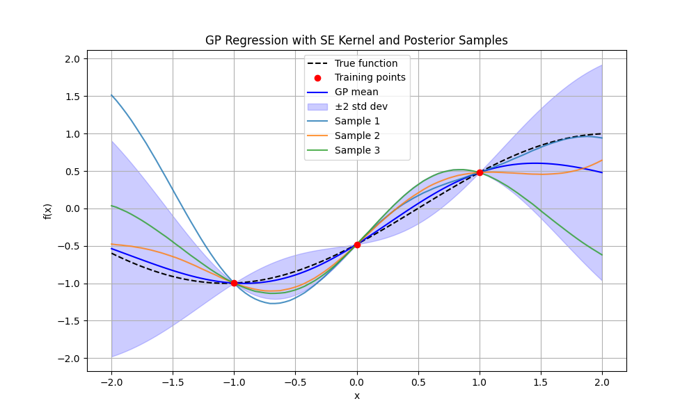
With that we are already able to sample our approximate \(F_*\) as a multivariate normal distribution, we get \(N\) points which correspond exactly to our test points.

rng = np.random.default_rng(0)
sample_functions = rng.multivariate_normal(mu, cov, 3)

Plots

GP Posterior Sample

Technical Details and Performance

Full implementation can be found here.

Numerical Stability

Even when we don’t assume any measurement noises it is prudent to add a slight diagonal offset to the top left and bottom right covariance matrix to improve numerical stability and matrix condition

K_XX = get_covariance_from_kernel(x_train, x_train) + 1e-6 * np.eye(n_train)
K_SS = get_covariance_from_kernel(xs, xs) + 1e-6 * np.eye(ns)

Matrix Inversion

Matrices should never be explicitly inverted (e.g. with np.linalg.inv) — instead, using the Cholesky decomposition is both significantly faster and more memory efficient. For a numerically stable implementation, see Rasmussen & Williams (2006), §2.2 Function space view.

Broadcasting for Kernel Application

A more efficient implementation of the kernel, using broadcasting

def get_covariance_from_kernel(X: np.ndarray, Y: np.ndarray) -> np.ndarray:
    X = X[:, np.newaxis]
	assert X.shape == (len(X), 1)
    Y = Y[np.newaxis, :]
	assert Y.shape == (1, len(Y))
    sq_dist = (X - Y) ** 2
	assert sq_dist.shape == (len(X), len(Y))
    return np.exp(-0.5 * sq_dist)

References

Rasmussen, C.E. & Williams, C.K.I. (2006). Gaussian Processes for Machine Learning. MIT Press. Online version
Bishop, C.M. (2006). Pattern Recognition and Machine Learning. Springer. Relevant sections: Chapter 6.1 (Gaussian Processes) and 6.4 (Bayesian Linear Regression).
Wikipedia – Gaussian Process
https://github.com/Daniel-Sinkin/DeepLearning/blob/main/visualisations/gaussian_process.py